Predicting Engine Failure using C-MAPSS data

As a Mechanical Engineer, I wished to combine the worlds of Engines and Machine Learning in a project. To that effect, I decided to use some data generated using the Modular Aero-Propulsion System Simulation (MAPSS), specifically it’s commercial version known as C-MAPSS.

The commercial versions, C-MAPSS and C-MAPSS40k, represent high-bypass engines capable of 90,000 lbf thrust and 40,000 lbf thrust, respectively.

This dataset was made available by NASA for research on prognostic/preventive maintenance of engines.

Background

Turbofan Engines are the kind of engines used in airplanes and jets. They work by sucking air into the front of the engine using a fan. From there, the engine compresses the air, mixes fuel with it, ignites the fuel/air mixture, and shoots it out the back of the engine, creating thrust.

Maintenance of these bad boys can get really expensive yet remains extremely important, as failure can result in catastrophes.

The aim of this model is to potentially:

->Provide critical information and an estimate of the health of an engine.

->Lead to cost savings by avoiding unscheduled maintenance.

->Increase equipment usage.

Engine Degradation Simulation

I used the Turbofan Engine Degradation Simulation Dataset.

From the website:

“Engine degradation simulation was carried out using C-MAPSS. Four different were sets simulated under different combinations of operational conditions and fault modes. Records several sensor channels to characterize fault evolution. The data set was provided by the Prognostics CoE at NASA Ames.”

“Data sets consist of multiple multivariate time series. Each data set is further divided into training and test subsets. Each time series is from a different engine ñ i.e., the data can be considered to be from a fleet of engines of the same type. Each engine starts with different degrees of initial wear and manufacturing variation which is unknown to the user. This wear and variation is considered normal, i.e., it is not considered a fault condition. There are three operational settings that have a substantial effect on engine performance. These settings are also included in the data. The data are contaminated with sensor noise.

The engine is operating normally at the start of each time series, and starts to degrade at some point during the series. In the training set, the degradation grows in magnitude until a predefined threshold is reached beyond which it is not preferable to operate the engine. In the test set, the time series ends some time prior to complete degradation.”

EDA

Data Set: FD001

Train trjectories: 100

Test trajectories: 100

Conditions: ONE (Sea Level)

Fault Modes: ONE (HPC Degradation)

Data Set: FD002

Train trjectories: 260

Test trajectories: 259

Conditions: SIX

Fault Modes: ONE (HPC Degradation)

Data Set: FD003

Train trjectories: 100

Test trajectories: 100

Conditions: ONE (Sea Level)

Fault Modes: TWO (HPC Degradation, Fan Degradation)

Data Set: FD004

Train trjectories: 248

Test trajectories: 249

Conditions: SIX

Fault Modes: TWO (HPC Degradation, Fan Degradation)

We have 4 datasets, each dataset further has a training and a testing subset.

Based on the information given, we know that the engines in the training set are operating normally in the beginning and have failed by the end.

Let’s look at some sensor readings to see if we can establish this through histograms. Let’s look at the Total Pressure at Outlet for the first 20 and the last 20 cycles.

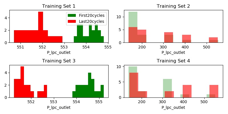
We see a clear delineation between the first and last 20 cycles of the engine in Training Sets 1 and 3. However, training sets 2 and 4 - the delineation is not as clear.

Looking at Fan Speed, we see a similar pattern.

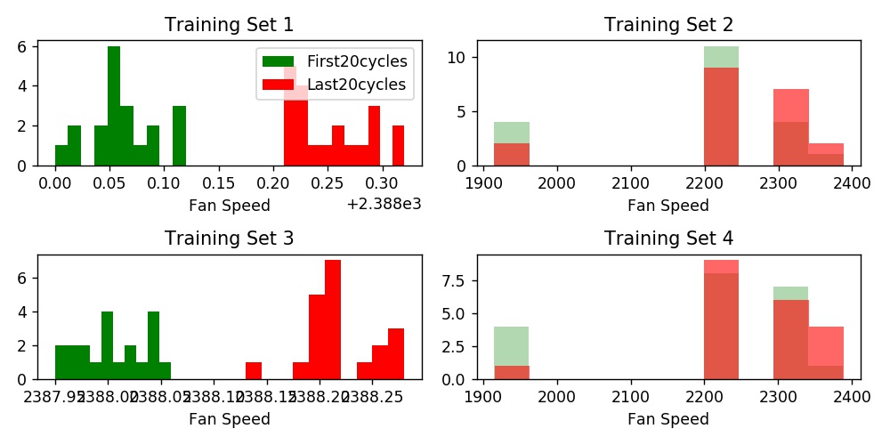
So what’s the difference between Training Sets 1 & 3 and 2 & 4?

The operating conditions (in BOLD above). Per the documentation provided with the data, Training sets 1 and 3 - all the engines are operating under just one condition while in training sets 2 and 4, the engines are operating under SIX different conditions.

While modeling, we will need to take this into account.

Modeling

1. KNN

2. Logistic regression

3. Support Vector Machines

4. Decision Trees

5. Bagging Classifier

6. Random Forest

Let’s walk through implementations of each of these to arrive at our best model.

1. KNN

To get started, I create a new column: ‘is_failing’ and append it to my existing dataframes. In this column, the first 20 cycles for each unit within the training data are labeled as 0 and the last 20 are labeled as 1.

I train the model on each of the training sets and compare it’s performance on the others.

Training Set 1:

Training Set 2:

Training Set 3:

Training Set 4:

Training Sets 1 and 3, as expected - operating under one condition - are not very predictive on the sets operating under 6 different conditions.

Training Sets 2 and 4, though are almost perfect at predicting engine failure in the other sets!

This is because, as can be seen in the histograms we made above, there is a very clear delineation between completely healthy engines (first 20 cycles) and engines that have failed (last 20 cycles), KNN is easily able to pick this out. This, however, is not very helpful as we are solving a solved problem.

Let’s explore the relationship between sensor readings of a healthy engine and one towards the end of it’s life.

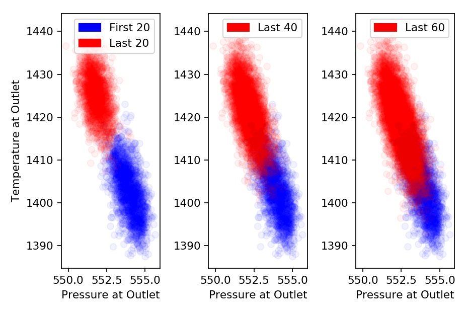
The scatter plot above compares Outlet Temperature and Outlet Pressure during the first 20 cycles and last 20, 40, and 60 cycles for all engines in Training Set 1.

Note how as we slide the window of our ‘failing’ engines to 40 and 60 cycles, overlap of sensor readings between healthy and failing engines increases.

Can we predict an engine is failing 60 cycles (hours) before it fails?

Moving forward, let’s make 2 sub-models using each of the techniques above. One for training sets operating under ONE condition and another for training sets operating under SIX conditions.

We expect our ONE condition model to do slightly worse over the four testing sets than the SIX condition model.

However, our ONE condition model returns an accuracy of ~88% while our SIX condition models returns an accuracy of ~83%.

That doesn’t seem right?

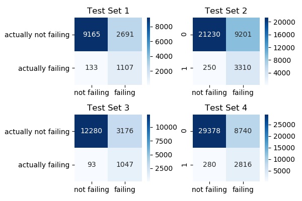
Let’s explore further through a confusion matrix.

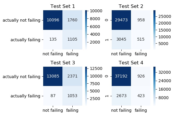
According to this, in Test Set 1:

Of a total of 11856 (10096+1760) healthy engines, our model identified 10096 engines correctly as ‘not failing’ (True Positives). It identified 1760 engines as ‘failing’ even though they were healthy (False negatives).

Of a total of 1240 (135+1105) failing engines, our model correctly identified 1105 engines correctly as ‘failing’ (True Negatives). It misidentified 135 bad engines as being healthy (False Positives).

The ratio of correctly identified healthy engines (True Positives) to the total number of engines identified as healthy (True Positives + False Positives) is called ‘Precision’. In Test Set 1, the precision is 98.6% (10096/10096+135).

The ratio of correctly identified healthy engines (True Positives) to the actual total number of healthy engines (True Positives + False Negatives) is called ‘Recall’. In Test Set 1, the recall is 85.15% (10096/10096+1760).

The ratio of correctly identified failing engines (True Negatives) to the actual total number of failing engines (True Negatives + False Positives) is called ‘Specificity’ or ‘True Negative Rate’. In Test Set 1, the specificity is 89.11% (1105/1105+135).

In this exercise of predicting engine failure, we are interested in maximizing our correct predictions of engines that are failing i.e. the metric that we will try to optimize for is going to be, specificity.

KNN ONE condition model - Specificity (%)

Test Set 1: 89.11

Test Set 2: 14.46

Test Set 3: 92.36

Test Set 4: 13.66

Mean: 52.39

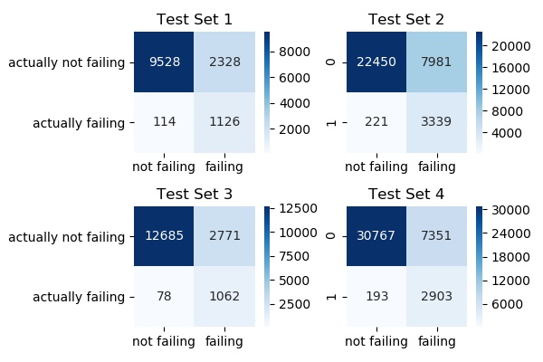
Looking at the confusion matrix for SIX condition models.

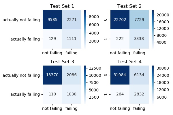
KNN SIX condition model - Specificity (%)

Test Set 1: 89.59

Test Set 2: 93.76

Test Set 3: 90.35

Test Set 4: 91.47

Mean: 91.29

So while at first glance, it might look like the ONE condition model was outperforming the SIX condition model, looking at it more deeply and taking into account the metric that we are interested in - we see that the SIX condition model does a lot better.

2. Logistic regression

Specificity (%)

Test Set 1: 93.70

Test Set 2: 94.52

Test Set 3: 88.42

Test Set 4: 87.79

Mean: 91.10

3. Support Vector Machines

Specificity (%)

Test Set 1: 93.54

Test Set 2: 94.38

Test Set 3: 88.24

Test Set 4: 87.53

Mean: 90.92

4. Decision Trees

Specificity (%)

Test Set 1: 89.27

Test Set 2: 92.97

Test Set 3: 91.84

Test Set 4: 90.95

Mean: 91.25

5. Bagging Classifier

Specificity (%)

Test Set 1: 90.80

Test Set 2: 93.79

Test Set 3: 93.15

Test Set 4: 93.76

Mean: 92.87

6. Random Forest

Specificity (%)

Test Set 1: 90.72

Test Set 2: 94.35

Test Set 3: 93.50

Test Set 4: 93.12

Mean: 92.92

Conclusion/Future Work

Based on the results above, we see that due to the nature of the problem - almost all our classifiers perform reasonably well. Our worst performing classifier, the Support Vector Machine model comes out with a mean specificity of 90.92% while our best performing classifier, the random forest model has a mean specificity of 92.92%. Not bad, at all!

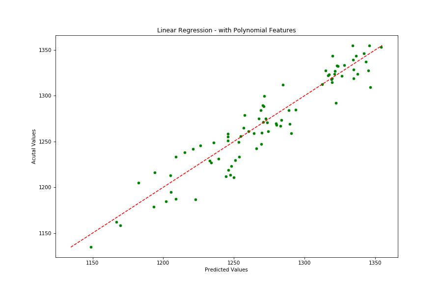
Seeing as how the data-set was setup to be used in a regression analysis, I’d like to create that model and compare it’s results with my classification models discussed above.

Linear Regression & The Price of Gold

What contributes to the price of a shiny metal?

Decided to use my new found Linear Regression and Web Scraping powers to find a relationship between the price of an ounce of Gold and the following features:

1. The ThomasRetuters Core Commodity Index Fund (CRB) This Index Fund is made up of 19 commodities - with 39% allocated to energy contracts, 41% to agriculture, 7% to precious metals and 13% to industrial metals.

2. Monthly Inflation Rate How much is USD worth today compared to how much it was worth a month ago?

3. M1 Money Supply How much USD has the Federal Reserve printed?

4. EURUSD How much USD does it take to buy 1 EUR?

After establishing these as my features, I decided to get my data.

–> Scraped the price of Gold using Selenium from this website.

–>Inflation Data was scraped using Selenium from this one.

–>The other websites were nice enough to provide a direct download link!

Analysis

Let’s look at the price of gold between August 2016 and April 2018.

Now, let’s look at all our features over the same period.

Do you see some trends? Good. Let’s see if we can find a nice little equation that captures this relationship.

Before we dive into actually finding our equation, Let’s find out-

How are these features related to the price of Gold?

From this correlation heat-map, we see that of our 4 features, EURUSD seems to be the most correlated to the price of Gold, followed by M1SL, inflation rate (negatively correlated) and lastly the CRB index.

Linear Regression

I start simple. Using the good old Ordinary Least Squares method, I get:

With an R^2 score of 0.67, and a Mean Absolute Error (MAE) of $28, while it’s not abysmal. It’s surely not very good. Also, notice how whenever the price is over $1300, my model does terribly.

Clearly there are some relationships that my model is not picking out on.

What if I try adding Polynomial Features into the mix? Basically, I’m giving my model permission to use features like EURUSD * M1 Money Supply or CRB Index^2.

My model immediately does better -

Note that here I am using 2nd degree Polynomial Features. My R^2 is up to 0.82 and MAE is down to $15.

Pretty neat huh? Clearly my chosen features have a relationship with the price of an ounce of gold! Yay!

What’s next?

The next step is to add a time series component to this analysis to ‘predict’ the future price given historical price. Start by trying some simple Auto-Regressive/Moving Average models. Maybe see how the recently released Facebook Prophet library fares. Once you know Linear Regression, the possibilities are endless!

**I will be uploading my notebook with all the code to achieve all of the above to my Github repo shortly! Stay tuned! **